Chapter 9 CMIP6 Models and CDO
9.1 CMIP6 models? What the F*** is that?
CMIP6 stands for Coupled Model Intercomparison Project (CMIP). These are climate models that simulate the physics, chemistry and biology of the atmosphere in detail (some of them!). The 2013 IPCC fifth assessment report (AR5) featured climate models from CMIP5, while the upcoming 2021 IPCC sixth assessment report (AR6) will feature new state-of-the-art CMIP6 models (more info in Carbon Brief website.)
The main goal is to set future climate scenarios based on future concentrations of greenhouse gases, aerosols and other climate forcings to project what might happen in the future.
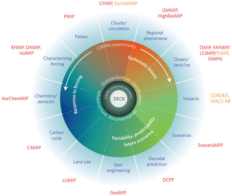
Figure 9.1: Schematic of the CMIP/CMIP6 experimental design
9.1.1 Most common climate scenarios
From CMIP5 version you will find those as RCPs (Representative Concentration Pathways) but for the new CMIP6 version they are called SSPs (Shared Socio‐Economic Pathways).
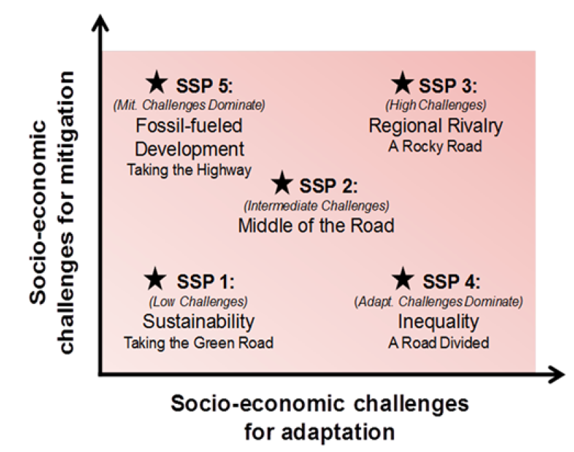
Figure 9.2: Overview of SSPs
Most commonly SSPs used (at least for me):
- SSP1(2.6): low challenges for mitigation (resource efficiency) and adaptation (rapid development)
- SSP2(4.5): intermediate challenges for mitigation
- SSP5(8.5): high challenges for mitigation (resource / fossil fuel intensive) and low for adaptation (rapid development)
9.1.2 Can I use those models?
Yes you can. They are free available at the Earth System Grid Federation. You will need an account to download models. Check this tutorial of how to create an account.
For now, let’s go through the website:
- Click here to open the ESGF website
- Go to the Nodes tab to explore the different ESGF-CoG nodes
- Click the NCI link, the Australia National Computational Infrastructure node
In the NCI node, go to collection and then click the CMIP6 link. This is the main website to download models. At your left you have several filters that you can play with, my advice is filter first for variable.
9.2 Variable Choice
There are a range of variables available from the GCM (General Circulation Model) outputs. In the file linked here you can explore the available variables. Each tab has different model variable on different time scales. The tabs are in alphabetical order. The ones starting with “O” are for Ocean, and then followed by the timescale (clim = climatology, day, dec = decade, mon = month, yr) (source: Mathematical Marine Ecology Welcome Book Chapter 9).
9.2.1 Let’s play with filters
From the left tab:
- click the + in the variable option. Select tos (ocean temperature on surface). Then click Search
- click the + in the Realm option. Select ocean and ocnBgChem. Then click Search
- click the + in the Frequency option. Select mon. Then click Search
- click the + in the Variant Label option. Select r1i1p1f1 (this is the most common ensemble). Then click Search
The ensemble names “r1i1p1”, “r2i1p1”, etc. in Variant Label indicate that the ensemble members differ only in their initial conditions (the model physics are the same for all ensemble members, but the members were initialized from different initial conditions out of the control simulation). Hence, the differences between the ensemble members represent internal variability.
- click the + in the Experiment ID option. In this option you will see every single Experiment/Simulation. For example, G1/G6/G7 are the geoengineering climate scenarios. Go to the bottom of the Experiment ID tab and click ssp126. Then click Search
- click the + in the Source ID option for the full model list and their Institution ID. Let’s click on ACCESS-CM2 model from the CSIRO. Then click Search
If you have follow the previous steps you should get a tab result similar to this:

(#fig:tab model example)ACCESS-CM2 SSP126
To download the model, just click on the List Files tab and then select HTTP Download
NOTE: if you are part of an Australian University you can request formal access to the NCI cluster gadi. CMIP6 models are under projects fs38 (CMIP6 Australian Data Publication) and oi10 (CMIP6 Replication Data). You can download models directly from the cluster on an average speed of ~100mb/s.
9.3 Working with CMIP6 netCDF files using CDO (Climate data operators)
Here I’m going to describe how to work with CDO if you work with CMIP6 climatic data. CMIP6 models came in netCDF file format and they are usually really messy to work in R (at least for me!). For example, the resolution of the CMIP6 NOAA model (ssp126) is 0.25°. Let say that you want to download that model for the thetao variable (sea temperature with depth). The size of that model is ~80gb. It will be really hard just to read that file in R.
The intention with this info (and scripts) is to provide a basic understanding of how you can use CDO to speed-up your netCDF file data manipulation. More info go directly to the Max Planck Institute CDO website
9.3.1 Installation Process
9.3.1.1 MacOS
I couldn’t install CDO from homebrew so I followed the instruction and downloaded MacPorts. MacPorts is an open-source community initiative to design an easy-to-use system for compiling, installing, and upgrading the command-line on the Mac operating system.
MacPorts website MacPorts download
After the installation (if you have admin rights) open the terminal and type:
port install cdo
If you don’t have admin rights, open the terminal and type:
sudo port install cdo and write your password
9.3.1.2 Windows 10
In the current windows 10 version(s) Microsoft included an Ubuntu 16.04 LTS embedded Linux. This environment offers a clean integration with the windows file systems and and the opportunity to install CDO via the native package manager of Ubuntu.
Install the Ubuntu app from the Microsoft Store application. Then open the Ubuntu terminal and type:
sudo apt-get install cdo and write your password
9.3.1.3 Linux
For Linux go to: Linux
9.3.2 Ncview: a netCDF visual browser
Browsing and browsing, I found a quick visual browser that allows you to explore netCDF files very easily: ncview. ncview is an easy to use netCDF file viewer for linux and OS X. It can read any netCDF file.
To install ncview, open the terminal and type:
OS X : port install ncview
Linux: sudo apt-get install ncview
9.3.3 Working with CDO and ncview
To work with CDO and ncview you will need to use the terminal command line. Open the Ubuntu app in Windows and the Terminal on OS X. Let’s create a folder in your desktop:
First, create a new folder in your desktop. In your command line type:
cd Desktop/(this will establish Desktop as your primary directory)mkdir z_test(this will create a folder called z_test in Desktop)cd z_test/(this will establish z_test as your primary directory)
If your are using Windows your desktop path should be located at /mnt/c/. Therefore, my Desktop should be at:
cd /mnt/c/Users/Isaac/Desktop/mkdir z_testcd z_test/
9.3.4 Files in directory
If you have the chance, please download this file. It is the EC-Earth3-Veg CMIP6 models for thetao (sea water with depth). Move that file into the z_test folder.
Because you have setting z_test as your directory in the terminal, we can use ncview to get a quick view of the model
- type
ls -lto see if the model is in your directory. You should get something like this:
(#fig:model directory)directory
- to view the model with ncview, in the terminal type
ncview thetao_Omon_EC-Earth3-Veg_ssp245_r1i1p1f1_gn_203401-203412.nc. You should see something like this: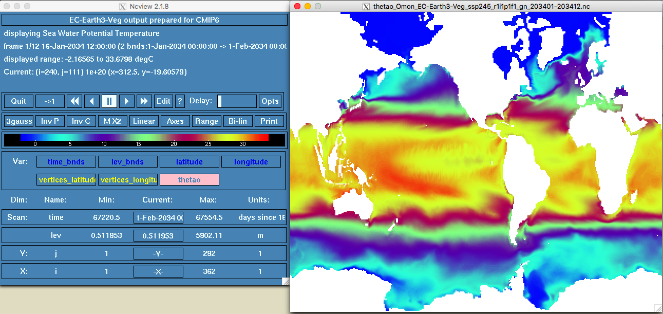
Figure 9.3: ncview example
- You can click the different options here. This model has long, lat, time and lev(or depth). You can press play and move the Delay option to check the different time settings (in this case months of the year 2034).
As you can see the model looks weird. That is because it has been originally created in curvilinear or circular resolution. We can check the file details using cdo. In the terminal type:
cdo -sinfov thetao_Omon_EC-Earth3-Veg_ssp245_r1i1p1f1_gn_203401-203412.nc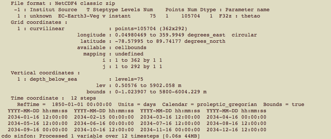
(#fig:model details)details
The model details are:
- Variable: thetao
- Horizontal component: resolution 362x292, which is ~ 1°x 0.5°
- Vertical component: 75 levels (i.e., depths)
- Time component: 12 steps (i.e., 12 months)
WE HAVE NOT EVEN OPENED R YET!!! :-)
9.3.5 Regridding with CDO
If you want to regrid and interpolate a netCDF file with CDO, the easiest way (for me!) is to create a standard grid file with the argument griddes.
To regrid a netCDF file using CDO you will have to use the argument remapbil, which is the stands for bilinear interpolation (there are other methods but this is the most conservative approach). CDO Syntax works like this:
- cdo -[function] input_file output_file
To regrid the file using bilinear interpolation in the terminal type:
cdo -remapbil,r360x180, thetao_Omon_EC-Earth3-Veg_ssp245_r1i1p1f1_gn_203401-203412.nc regrid_file.nc
To check the model NEW details just type cdo -sinfov regrid_file.nc:
- Variable: thetao
- Horizontal component: resolution 362x180 or 1°x 1°
- Vertical component: 75 levels (i.e., depths)
- Time component: 12 steps (i.e., 12 months)
Let’s see how our new model looks now. In the terminal type:
ncview regrid_file.nc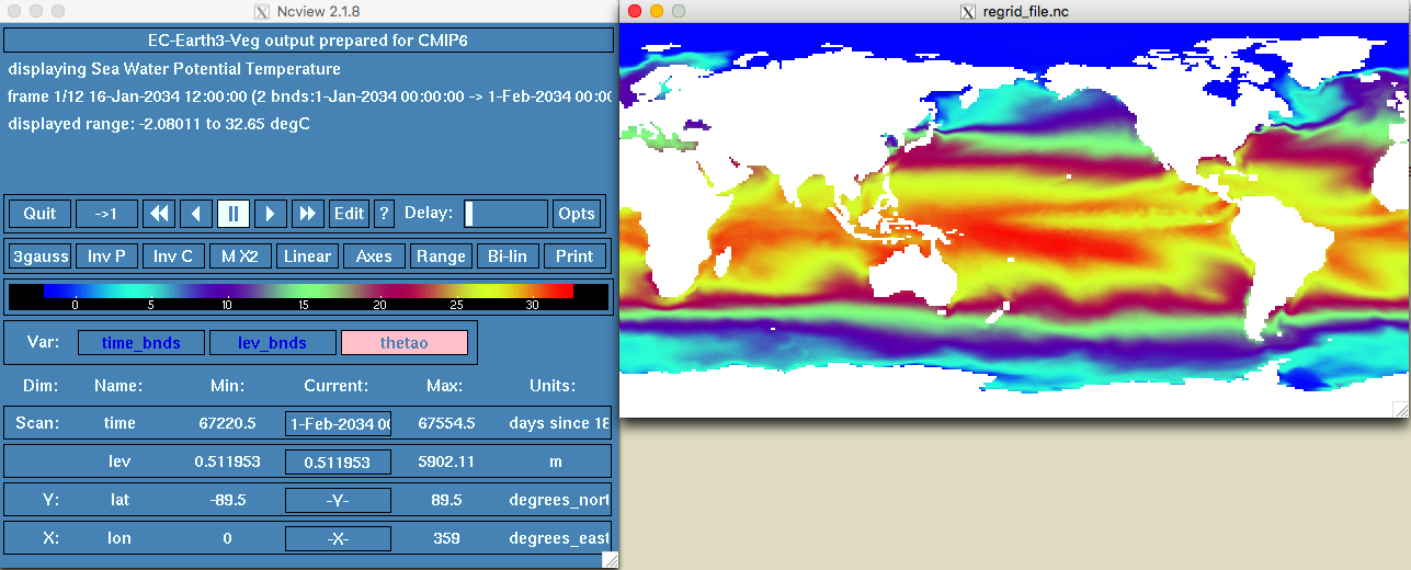
(#fig:new model details)regrid model
OK so this looks better!!!
9.4 CDO with multiple input models/files
The previous “regridding process” works fine if you have one or two netCDF files. However, if you have multiple netCDF files/models (which is most cases of CMIP6 models) the best way to do it is to write a simple (or not) shell script to iterate the same process for every file/model. The other alternative is to use R to call CDO through the system() function.
Look the components of the shell file cdo_rg.sh from my personal Github repo
9.5 CDO extra functions
CDO is more than just regridding. There are several things that you can explore. Some interesting functions that I’ve used a lot are:
cdo -yearmeancalculates the annual mean of a monthly data input netCDF filecdo -yearmincalculates the annual min of a monthly data input netCDF filecdo -yearmaxcalculates the annual max of a monthly data input netCDF filecdo -ensmeancalculates the ensemble mean of several netCDF files. If your input files are different models, this function will estimate a mean of all those modelscdo -vertmeancalculates the vertical mean for netCDF with olevel (i.e., depth)cdo -mergetimemerge all the netCDF files in your directory
To use those argument remember just type in the terminal:
- cdo -[function] input_file output_file