Plot solution comparison

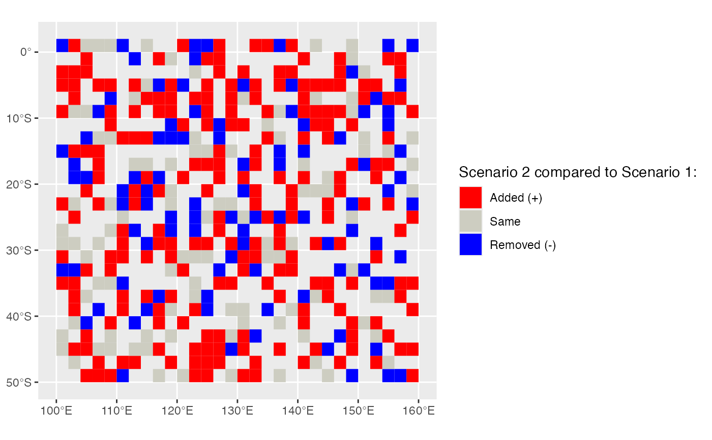
Conservation planning often requires the comparison of the outputs of the solutions of different conservation problems. One way to compare solutions is by spatially visualising the different planning units that were selected in two separate solutions to conservation problems. splnr_plot_comparison() allows to map the differences of two solutions in customisable way using ggplot2. This function requires two separate sf objects each containing a solution_1 column indicating the binary solution (selected vs not selected) of a prioritizr conservation problem. It outputs a ggobject and can be combined with the spatialplanr function splnr_gg_add().

Usage

splnr_plot_comparison(
  soln1,
  soln2,
  legendTitle = "Scenario 2 compared to Scenario 1:"
)

Arguments

soln1

The first prioritizr solution

soln2

The second prioritizr solution

legendTitle

A character value for the title of the legend. Can be empty ("").

Value

A ggplot object of the plot

Examples

# 30 % target for problem/solution 1
dat_problem <- prioritizr::problem(dat_species_bin %>% dplyr::mutate(Cost = runif(n = dim(.)[[1]])),
  features = c("Spp1", "Spp2", "Spp3", "Spp4", "Spp5"),
  cost_column = "Cost"
) %>%
  prioritizr::add_min_set_objective() %>%
  prioritizr::add_relative_targets(0.3) %>%
  prioritizr::add_binary_decisions() %>%
  prioritizr::add_default_solver(verbose = FALSE)

dat_soln <- dat_problem %>%
  prioritizr::solve.ConservationProblem()

# 50 % target for problem/solution 2
dat_problem2 <- prioritizr::problem(
  dat_species_bin %>%
    dplyr::mutate(Cost = runif(n = dim(.)[[1]])),
  features = c("Spp1", "Spp2", "Spp3", "Spp4", "Spp5"),
  cost_column = "Cost"
) %>%
  prioritizr::add_min_set_objective() %>%
  prioritizr::add_relative_targets(0.5) %>%
  prioritizr::add_binary_decisions() %>%
  prioritizr::add_default_solver(verbose = FALSE)

dat_soln2 <- dat_problem2 %>%
  prioritizr::solve.ConservationProblem()

(splnr_plot_comparison(dat_soln, dat_soln2))