5 Spatial Data
The aim of this tutorial is to provide a worked example of how vector-based data can be used to develop conservation prioritizations using the prioritizr R package. The dataset used in this tutorial was originally a subset of a larger spatial prioritization project performed under contract to Australia’s Department of Environment and Water Resources (Klein et al. 2007).
This dataset contains two items.
First, a spatial planning unit layer that has an attribute table which contains three columns: integer unique identifiers (“id”), unimproved land values (“cost”), and their existing level of protection (“status”). Units with 50 % or more of their area contained in protected areas are associated with a status of 2, otherwise they are associated with a value of 0.
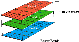
The second item in this dataset is the raster-based feature data. Specifically, the feature data is expressed as a stack of rasters (termed a
RasterStackobject). Here each layer in the stack represents the distribution of a different vegetation class in Tasmania, Australia. There are 62 vegetation classes in total. For a given layer, pixel values indicate the presence (value of 1) or absence (value of 0) of the vegetation class in an area.
First, load the required packages and the data.
5.1 Data import
# load packages
library(prioritizr)
library(prioritizrdata)
library(sf)
library(rgdal)
library(raster)
library(rgeos)
library(mapview)
library(units)
library(scales)
library(assertthat)
library(gridExtra)
library(dplyr)
## Some of this data is built in to the Prioritizr package, but it is lower resolution so we use that in the data/ folder.
# load planning unit data
# data(tas_pu) # SpatialPolygonsDataFrame # If raw, use readOGR(filename)

# load conservation feature data
# data(tas_features) # RasterStack # If raw, use stack(filename)

albers <- "+proj=aea +lat_1=-18 +lat_2=-36 +lat_0=0 +lon_0=132 +x_0=0 +y_0=0 +ellps=GRS80 +towgs84=0,0,0,0,0,0,0 +units=m +no_defs"

tas_pu <- readOGR("data/pu.shp")
## OGR data source with driver: ESRI Shapefile
## Source: "/Users/jason/GitHub/SpatialPlanning_Workshop2021/data/pu.shp", layer: "pu"
## with 1130 features
## It has 5 fields
tas_features <- stack("data/vegetation.tif")
proj4string(tas_pu) <- albers # There is a problem with projection so we re-add it here
proj4string(tas_features) <- albers # There is a problem with projection so we re-add it here

tas_pu$locked_out[1:500] <- FALSE # There is a problem later on so we remove some of the locked out areas to improve chance of a solution
tas_pu$locked_in <- as.logical(tas_pu$locked_in) # Convert to logical
tas_pu$locked_out <- as.logical(tas_pu$locked_out) # Convert to logical

# A function to plot the solution.
plot_solution <- function(s){
  s$solution_1 <- factor(s$solution_1)
  plot(st_as_sf(s[, "solution_1"]), pal = c("grey90", "darkgreen"), main = "Solution 1")
}
5.2 Planning unit data
The planning unit data contains spatial data describing the geometry for each planning unit and attribute data with information about each planning unit (e.g. cost values). Let’s investigate the tas_pu object. The attribute data contains 5 columns with contain the following information:
-
id: unique identifiers for each planning unit -
cost: acquisition cost values for each planning unit (millions of Australian dollars). -
status: status information for each planning unit (only relevant with Marxan) -
locked_in: logical values (i.e.TRUE/FALSE) indicating if planning units are covered by protected areas or not. -
locked_out: logical values (i.e.TRUE/FALSE) indicating if planning units cannot be managed as a protected area because they contain are too degraded.
# print a short summary of the data
print(tas_pu)
## class : SpatialPolygonsDataFrame
## features : 1130
## extent : 1080623, 1399989, -4840595, -4497092 (xmin, xmax, ymin, ymax)
## crs : +proj=aea +lat_0=0 +lon_0=132 +lat_1=-18 +lat_2=-36 +x_0=0 +y_0=0 +ellps=GRS80 +units=m +no_defs
## variables : 5
## names : id, cost, status, locked_in, locked_out
## min values : 1, 0.192488262910798, 0, 0, 0
## max values : 1130, 61.9272727272727, 2, 1, 1
# plot the planning unit data
plot(tas_pu)
# print the structure of object
str(tas_pu, max.level = 2)
## Formal class 'SpatialPolygonsDataFrame' [package "sp"] with 5 slots
## ..@ data :'data.frame': 1130 obs. of 5 variables:
## ..@ polygons :List of 1130
## ..@ plotOrder : int [1:1130] 217 973 506 645 705 975 253 271 704 889 ...
## ..@ bbox : num [1:2, 1:2] 1080623 -4840595 1399989 -4497092
## .. ..- attr(*, "dimnames")=List of 2
## ..@ proj4string:Formal class 'CRS' [package "sp"] with 1 slot
# print the class of the object
class(tas_pu)
## [1] "SpatialPolygonsDataFrame"
## attr(,"package")
## [1] "sp"
# print the slots of the object
slotNames(tas_pu)
## [1] "data" "polygons" "plotOrder" "bbox" "proj4string"
# print the geometry for the 80th planning unit
tas_pu@polygons[[80]]
## An object of class "Polygons"
## Slot "Polygons":
## [[1]]
## An object of class "Polygon"
## Slot "labpt":
## [1] 1289177 -4558185
##
## Slot "area":
## [1] 1060361
##
## Slot "hole":
## [1] FALSE
##
## Slot "ringDir":
## [1] 1
##
## Slot "coords":
## [,1] [,2]
## [1,] 1288123 -4558431
## [2,] 1287877 -4558005
## [3,] 1288177 -4558019
## [4,] 1288278 -4558054
## [5,] 1288834 -4558038
## [6,] 1289026 -4557929
## [7,] 1289168 -4557928
## [8,] 1289350 -4557790
## [9,] 1289517 -4557744
## [10,] 1289618 -4557773
## [11,] 1289836 -4557965
## [12,] 1290000 -4557984
## [13,] 1290025 -4557987
## [14,] 1290144 -4558168
## [15,] 1290460 -4558431
## [16,] 1288123 -4558431
##
##
##
## Slot "plotOrder":
## [1] 1
##
## Slot "labpt":
## [1] 1289177 -4558185
##
## Slot "ID":
## [1] "79"
##
## Slot "area":
## [1] 1060361
# print the coordinate reference system
print(tas_pu@proj4string)
## CRS arguments:
## +proj=aea +lat_0=0 +lon_0=132 +lat_1=-18 +lat_2=-36 +x_0=0 +y_0=0 +ellps=GRS80 +units=m +no_defs
# print number of planning units (geometries) in the data
nrow(tas_pu)
## [1] 1130
# print the first six rows in the attribute data
head(tas_pu@data)
## id cost status locked_in locked_out
## 0 1 60.24638 0 FALSE FALSE
## 1 2 19.86301 0 FALSE FALSE
## 2 3 59.68051 0 FALSE FALSE
## 3 4 32.41614 0 FALSE FALSE
## 4 5 26.17706 0 FALSE FALSE
## 5 6 51.26218 0 FALSE FALSE
# print the first six values in the cost column of the attribute data
head(tas_pu$cost)
## [1] 60.24638 19.86301 59.68051 32.41614 26.17706 51.26218
# print the highest cost value
max(tas_pu$cost)
## [1] 61.92727
# print the smallest cost value
min(tas_pu$cost)
## [1] 0.1924883
# print average cost value
mean(tas_pu$cost)
## [1] 25.13536
# plot a map of the planning unit cost data
spplot(tas_pu, "cost")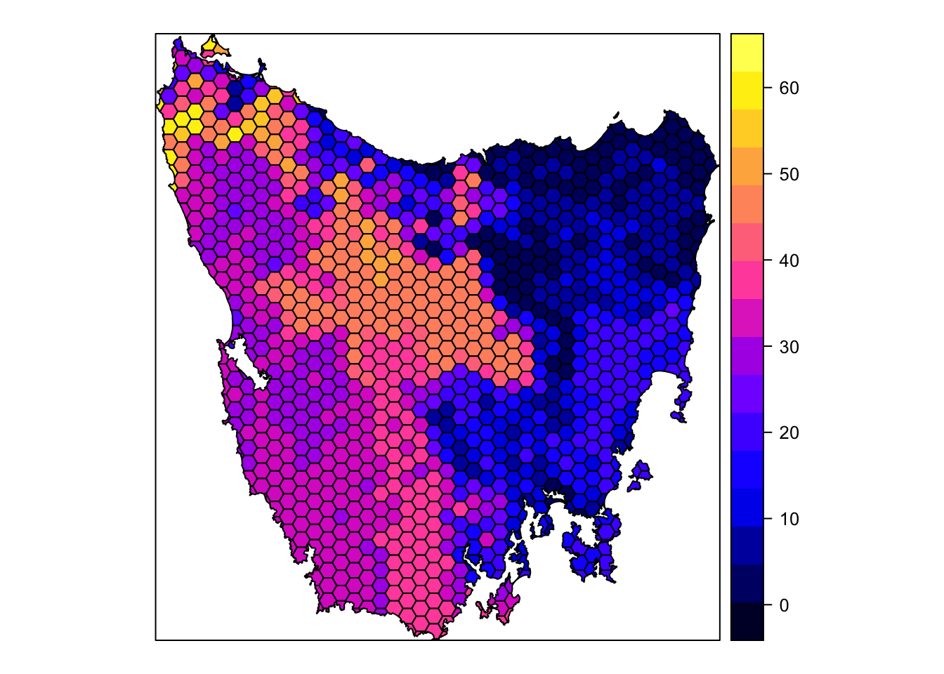
# plot an interactive map of the planning unit cost data
mapview(tas_pu, zcol = "cost")
Now, you can try and answer some questions about the planning unit data.
- How many planning units are in the planning unit data?
- What is the highest cost value?
- How many planning units are covered by the protected areas (hint:
sum(x))? - What is the proportion of the planning units that are covered by the protected areas (hint:
mean(x))? - How many planning units are highly degraded (hint:
sum(x))? - What is the proportion of planning units are highly degraded (hint:
mean(x))? - Can you verify that all values in the
locked_inandlocked_outcolumns are zero or one (hint:min(x)andmax(x))?. - Can you verify that none of the planning units are missing cost values (hint:
all(is.finite(x)))?. - Can you very that none of the planning units have duplicated identifiers? (hint:
sum(duplicated(x)))? - Is there a spatial pattern in the planning unit cost values (hint: use
spplotto make a map). - Is there a spatial pattern in where most planning units are covered by protected areas (hint: use
spplotto make a map).
5.3 Vegetation data
The vegetation data describes the spatial distribution of 62 vegetation classes in the study area. This data is in a raster format and so the data are organized using a square grid comprising square grid cells that are each the same size. In our case, the raster data contains multiple layers (also called “bands”) and each layer corresponds to a spatial grid with exactly the same area and has exactly the same dimensionality (i.e. number of rows, columns, and cells).
In this dataset, there are 62 different regular spatial grids layered on top of each other – with each layer corresponding to a different vegetation class – and each of these layers contains a grid with 343 rows, 320 columns, and 109760 cells.
Within each layer, each cell corresponds to a 1 by 1 km square. The values associated with each grid cell indicate the (one) presence or (zero) absence of a given vegetation class in the cell.
Let’s explore the vegetation data.
# print a short summary of the data
print(tas_features)
## class : RasterStack
## dimensions : 343, 320, 109760, 62 (nrow, ncol, ncell, nlayers)
## resolution : 1000, 1000 (x, y)
## extent : 1080496, 1400496, -4841217, -4498217 (xmin, xmax, ymin, ymax)
## crs : +proj=aea +lat_0=0 +lon_0=132 +lat_1=-18 +lat_2=-36 +x_0=0 +y_0=0 +ellps=GRS80 +units=m +no_defs
## names : vegetation.1, vegetation.2, vegetation.3, vegetation.4, vegetation.5, vegetation.6, vegetation.7, vegetation.8, vegetation.9, vegetation.10, vegetation.11, vegetation.12, vegetation.13, vegetation.14, vegetation.15, ...
## min values : 0, 0, 0, 0, 0, 0, 0, 0, 0, 0, 0, 0, 0, 0, 0, ...
## max values : 1, 1, 1, 1, 1, 1, 1, 1, 1, 1, 1, 1, 1, 1, 1, ...
# plot a map of the 36th vegetation class
plot(tas_features[[36]])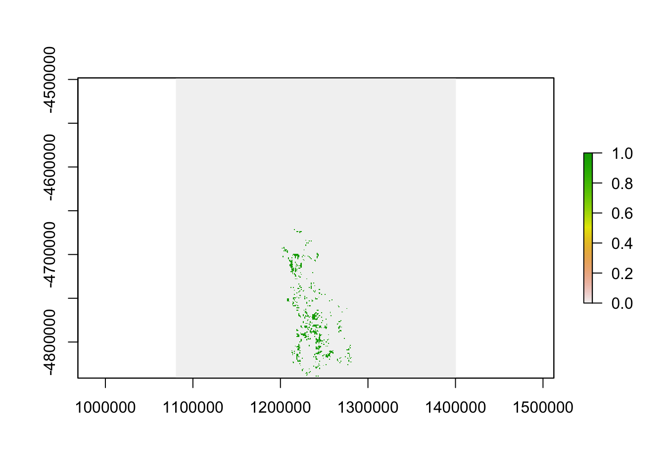
# plot an interactive map of the 36th vegetation class
mapview(tas_features[[36]])
# print number of rows in the data
nrow(tas_features)
## [1] 343
# print number of columns  in the data
ncol(tas_features)
## [1] 320
# print number of cells in the data
ncell(tas_features)
## [1] 109760
# print number of layers in the data
nlayers(tas_features)
## [1] 62
# print  resolution on the x-axis
xres(tas_features)
## [1] 1000
# print resolution on the y-axis
yres(tas_features)
## [1] 1000
# print spatial extent of the grid, i.e. coordinates for corners
extent(tas_features)
## class : Extent
## xmin : 1080496
## xmax : 1400496
## ymin : -4841217
## ymax : -4498217
# print the coordinate reference system
print(tas_features@crs)
## CRS arguments:
## +proj=aea +lat_0=0 +lon_0=132 +lat_1=-18 +lat_2=-36 +x_0=0 +y_0=0 +ellps=GRS80 +units=m +no_defs
# print a summary of the first layer in the stack
print(tas_features[[1]])
## class : RasterLayer
## band : 1 (of 62 bands)
## dimensions : 343, 320, 109760 (nrow, ncol, ncell)
## resolution : 1000, 1000 (x, y)
## extent : 1080496, 1400496, -4841217, -4498217 (xmin, xmax, ymin, ymax)
## crs : +proj=aea +lat_0=0 +lon_0=132 +lat_1=-18 +lat_2=-36 +x_0=0 +y_0=0 +ellps=GRS80 +units=m +no_defs
## source : /Users/jason/GitHub/SpatialPlanning_Workshop2021/data/vegetation.tif
## names : vegetation.1
## values : 0, 1 (min, max)
# print the value in the 800th cell in the first layer of the stack
print(tas_features[[1]][800])
##
## 0
# print the value of the cell located in the 30th row and the 60th column of
# the first layer
print(tas_features[[1]][30, 60])
##
## 0
# calculate the sum of all the cell values in the first layer
cellStats(tas_features[[1]], "sum")
## [1] 36
# calculate the maximum value of all the cell values in the first layer
cellStats(tas_features[[1]], "max")
## [1] 1
# calculate the minimum value of all the cell values in the first layer
cellStats(tas_features[[1]], "min")
## [1] 0
# calculate the mean value of all the cell values in the first layer
cellStats(tas_features[[1]], "mean")
## [1] 0.0003279883
# calculate the maximum value in each layer
as_tibble(data.frame(max = cellStats(tas_features, "max")))
## # A tibble: 62 x 1
## max
## <dbl>
## 1 1
## 2 1
## 3 1
## 4 1
## 5 1
## 6 1
## 7 1
## 8 1
## 9 1
## 10 1
## # … with 52 more rowsNow, you can try and answer some questions about the vegetation data.
- What part of the study area is the 51st vegetation class found in (hint: make a map)?
- What proportion of cells contain the 12th vegetation class?
- Which vegetation class is present in the greatest number of cells?
- The planning unit data and the vegetation data should have the same coordinate reference system. Can you check if they are the same?