Plot correlation matrices

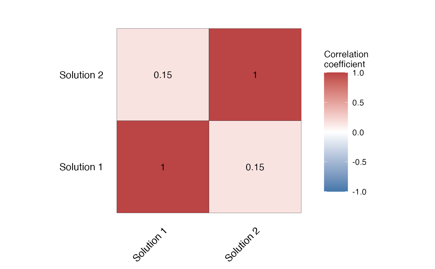
Conservation planning often requires the comparison of the outputs of the solutions of different conservation problems. One way to compare solutions is by correlating the solutions using Cohen's Kappa. splnr_plot_corrMat() allows to visualize the correlation matrix of the different solutions (for example produced with the spatialplanr function splnr_get_kappaCorrData()).

Usage

splnr_plot_corrMat(
  x,
  colourGradient = c("#BB4444", "#FFFFFF", "#4477AA"),
  legendTitle = "Correlation \ncoefficient",
  AxisLabels = NULL,
  plotTitle = ""
)

Arguments

x

A correlation matrix of prioritizr solutions

colourGradient

A list of three colour values for high positive, no and high negative correlation

legendTitle

A character value for the title of the legend. Can be empty ("").

AxisLabels

A list of labels of the solutions to be correlated (Default: NULL). Length needs to match number of correlated solutions.

plotTitle

A character value for the title of the plot. Can be empty ("").

Value

A ggplot object of the plot

Examples

# 30 % target for problem/solution 1
dat_problem <- prioritizr::problem(dat_species_bin %>% dplyr::mutate(Cost = runif(n = dim(.)[[1]])),
  features = c("Spp1", "Spp2", "Spp3", "Spp4", "Spp5"),
  cost_column = "Cost"
) %>%
  prioritizr::add_min_set_objective() %>%
  prioritizr::add_relative_targets(0.3) %>%
  prioritizr::add_binary_decisions() %>%
  prioritizr::add_default_solver(verbose = FALSE)

dat_soln <- dat_problem %>%
  prioritizr::solve.ConservationProblem()

# 50 % target for problem/solution 2
dat_problem2 <- prioritizr::problem(
  dat_species_bin %>%
    dplyr::mutate(Cost = runif(n = dim(.)[[1]])),
  features = c("Spp1", "Spp2", "Spp3", "Spp4", "Spp5"),
  cost_column = "Cost"
) %>%
  prioritizr::add_min_set_objective() %>%
  prioritizr::add_relative_targets(0.5) %>%
  prioritizr::add_binary_decisions() %>%
  prioritizr::add_default_solver(verbose = FALSE)

dat_soln2 <- dat_problem2 %>%
  prioritizr::solve.ConservationProblem()

CorrMat <- splnr_get_kappaCorrData(list(dat_soln, dat_soln2), name_sol = c("soln1", "soln2"))
#> New names:
#> • `soln1` -> `soln1...1`
#> • `soln1` -> `soln1...2`
#> New names:
#> • `soln2` -> `soln2...1`
#> • `soln2` -> `soln2...2`
#> New names:
#> • `` -> `...1`
#> • `` -> `...2`

(splnr_plot_corrMat(CorrMat, AxisLabels = c("Solution 1", "Solution 2")))
#> Scale for fill is already present.
#> Adding another scale for fill, which will replace the existing scale.
#> Scale for x is already present.
#> Adding another scale for x, which will replace the existing scale.